Heat transfer

Auto-generated 2026-10-17 09:01 UTC  ·  12 plots

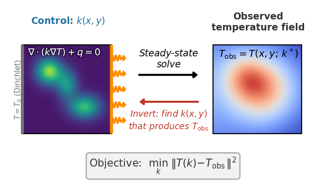
Invert for the conductivity field of a slab from its temperature, differentiating through a steady heat-conduction solve.

Inferring conductivity from temperature. Given the temperature field of a heated slab, where is the material conductive? We answer this inverse problem by differentiating through a steady heat-conduction solve.

The conductivity of a quasi-2D slab follows the SIMP law (\(p=3\)) \(k_\text{eff}(\rho) = k_\min + (k_\max - k_\min)\,\rho^3\) in the element density \(\rho\). The optimization experiment recovers a two-Gaussian density field from the temperature it produces, starting from a uniform field and minimizing \(\lVert T(\rho) - T_\text{target} \rVert^2\) with L-BFGS. The forward and gradient experiments compare solvers on the thermal compliance \(C = \oint_\Gamma q_n\,T\,d\Gamma\), the work done by the heat flux on the temperature field, and on its sensitivity to \(\rho\). Two further gradient experiments check the derivative of a temperature misfit with respect to a volumetric heat source \(f(\mathbf{x})\).

How these results were produced

These are example results, produced automatically on GitHub Actions runners and refreshed on every release. Each solver runs on its intended device: GPU-capable solvers on a Tesla T4 GPU node, CPU-only solvers (OpenFOAM, INS.jl, deal.II, FEniCS, Firedrake, TopOpt.jl) on a separate CPU node, whose processor model can differ between runs. Accuracy and gradient metrics are hardware-independent and reproducible. Wall-clock numbers reflect commodity cloud hardware and can vary by 10–15% between runs, so read them for relative scaling between solvers rather than as absolute timings. For numbers that reflect your setup, run the benchmarks yourself on your target hardware.

Boundary conditions

Quasi-2D heated slab on domain \([0,2]\times[0,1]\) (a single HEX8 layer, \(n_z=1\)). The slab thickness \(L_z\) scales with the in-plane element size (\(L_z = L_x/n_x\)) so the elements stay roughly cubic under refinement, keeping the linear system well-conditioned; \(Q_\text{total}\) is thus a flux per unit slab depth. Dirichlet: all nodes at \(x=0\) held at \(T=0\) (fixed temperature). Neumann (uniform): uniform heat flux \(Q_\text{total}\) over the right face (\(x=2\)). Neumann (hot-spot): flux concentrated on the central \(1/3\) stripe in \(y\) (\(L_y/3 \le y \le 2L_y/3\)) at the right face, used by the physical-laws check.

Initial Conditions

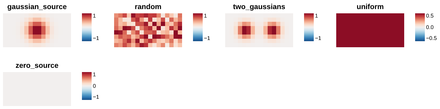
Visualisation of each initial condition (the starting field a run is launched from) available for this problem. IC plots are generated without running any solver.

Settings

Gaussian Source

{
  "nx": 16,
  "ny": 8,
  "nz": 1,
  "amplitude": 1.0,
  "cx": 0.5,
  "cy": 0.5,
  "sigma": 0.2
}

Random

{
  "rho_0": 0.5,
  "noise": 0.3,
  "nx": 16,
  "ny": 8,
  "nz": 1,
  "seed": 0
}

Two Gaussians

{
  "nx": 16,
  "ny": 8,
  "nz": 1
}

Uniform

{
  "rho_0": 0.5,
  "nx": 16,
  "ny": 8,
  "nz": 1
}

Zero Source

{
  "nx": 16,
  "ny": 8,
  "nz": 1
}

Forward

Is the prediction right? Forward-pass benchmarks check each solver’s output against a trusted reference (and an analytic solution where one exists): inter-solver agreement, field-level diagnostics, and long-run stability.

Agreement

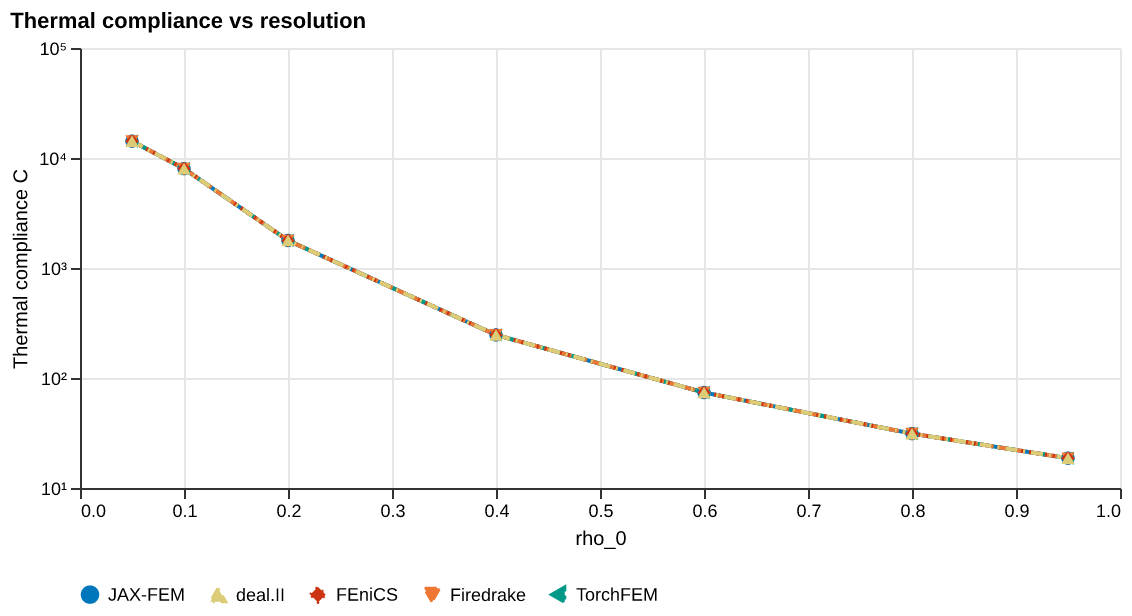
Thermal compliance \(C\) vs uniform element density \(\rho_0\) at fixed \(N\); compares solvers on a log scale.

Settings

Sweeps rho_0 ∈ {0.05, 0.1, 0.2, 0.4, 0.6, 0.8, 0.95}

{
  "ic": {
    "name": "uniform",
    "seed": 0
  },
  "physics": {
    "nx": 16,
    "ny": 8,
    "nz": 1,
    "Lx": 2.0,
    "Ly": 1.0,
    "Q_total": 1.0,
    "rho_0": 0.05
  },
  "sweep": {
    "key": "rho_0",
    "values": [
      0.05,
      0.1,
      0.2,
      0.4,
      0.6,
      0.8,
      0.95
    ]
  }
}

Baseline

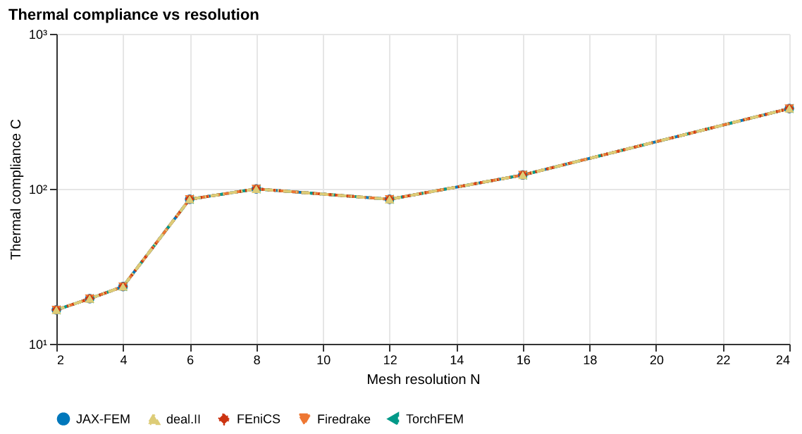
Thermal compliance \(C\) vs mesh resolution \(N\) with random density; compares FV and FEM solvers across refinements.

Settings

Sweeps N ∈ {2, 3, 4, 6, 8, 12, 16, 24}

{
  "ic": {
    "name": "random",
    "seed": 0
  },
  "physics": {
    "N": 2,
    "nz": 1,
    "Lx": 2.0,
    "Ly": 1.0,
    "Q_total": 1.0
  },
  "sweep": {
    "key": "N",
    "values": [
      2,
      3,
      4,
      6,
      8,
      12,
      16,
      24
    ]
  }
}

Physical Laws

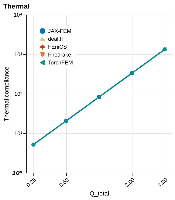
Thermal compliance \(C\) vs total heat flux \(Q_\mathrm{total}\) at fixed \(N\) and \(\rho_0\) with a hot-spot BC; shown on log-log axes.

Settings

Sweeps Q_total ∈ {0.25, 0.5, 1.0, 2.0, 4.0}

{
  "ic": {
    "name": "uniform",
    "seed": 0
  },
  "physics": {
    "N": 16,
    "nz": 1,
    "Lx": 2.0,
    "Ly": 1.0,
    "rho_0": 0.5,
    "hot_spot": true,
    "Q_total": 0.25
  },
  "sweep": {
    "key": "Q_total",
    "values": [
      0.25,
      0.5,
      1.0,
      2.0,
      4.0
    ]
  },
  "diagnostics": {
    "thermal_compliance": "<callable _get_thermal_compliance>"
  }
}

Source Baseline

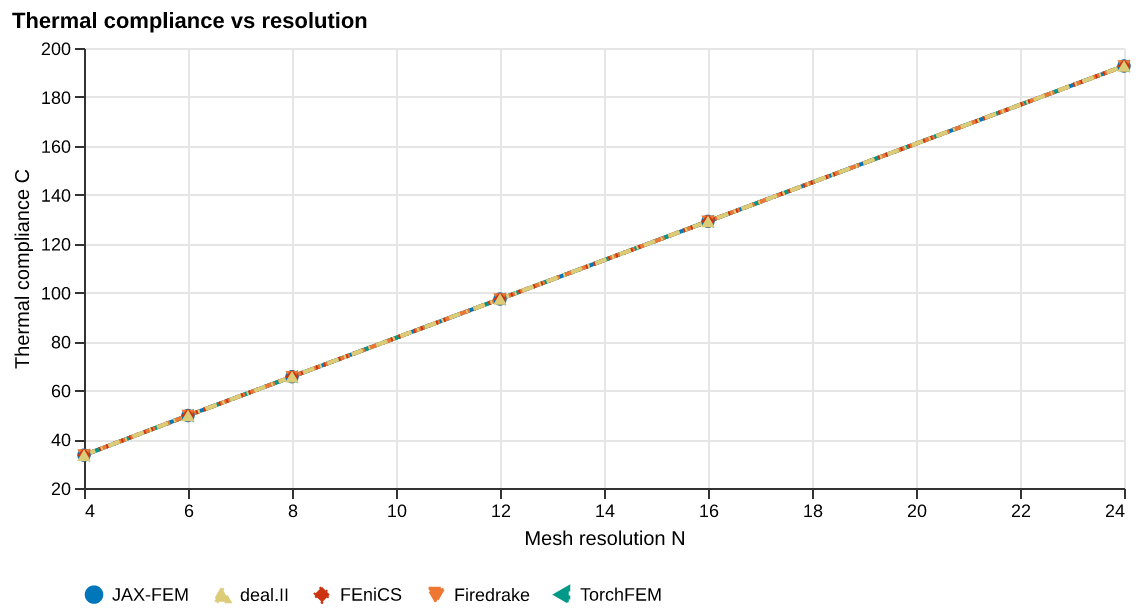
Thermal compliance \(C\) vs mesh resolution \(N\) with a Gaussian source field; compares solvers across refinements.

Settings

Sweeps N ∈ {4, 6, 8, 12, 16, 24}

{
  "ic": {
    "name": "gaussian_source"
  },
  "physics": {
    "N": 4,
    "nz": 1,
    "Lx": 2.0,
    "Ly": 1.0,
    "rho_0": 0.5,
    "ic_field": "source"
  },
  "sweep": {
    "key": "N",
    "values": [
      4,
      6,
      8,
      12,
      16,
      24
    ]
  }
}

Source Linearity

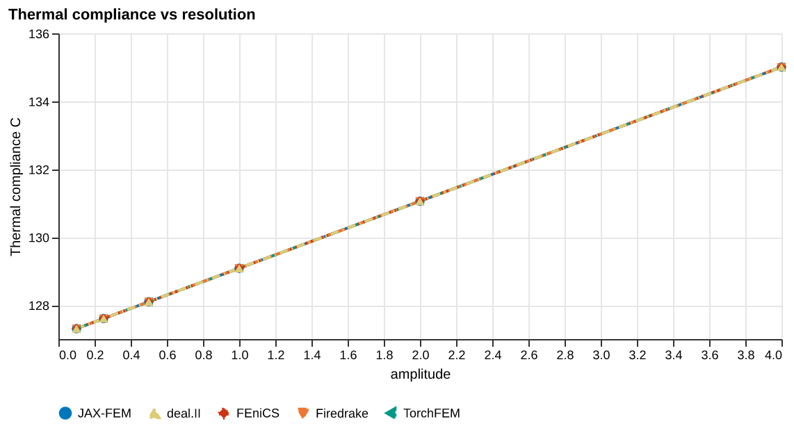
Thermal compliance \(C\) vs source amplitude at fixed mesh; compares solvers on log-log axes.

Settings

Sweeps amplitude ∈ {0.1, 0.25, 0.5, 1.0, 2.0, 4.0}

{
  "ic": {
    "name": "gaussian_source"
  },
  "physics": {
    "nx": 16,
    "ny": 8,
    "nz": 1,
    "Lx": 2.0,
    "Ly": 1.0,
    "rho_0": 0.5,
    "ic_field": "source",
    "amplitude": 0.1
  },
  "sweep": {
    "key": "amplitude",
    "values": [
      0.1,
      0.25,
      0.5,
      1.0,
      2.0,
      4.0
    ]
  }
}

Solver ranking

Solver	Mean rel. error
deal.II	1.74e-08
FEniCS	1.74e-08
Firedrake	1.74e-08
JAX-FEM	1.74e-08
torch-fem	1.74e-08

Ranked by mean relative error against the reference solution (lower is more accurate).

Cost

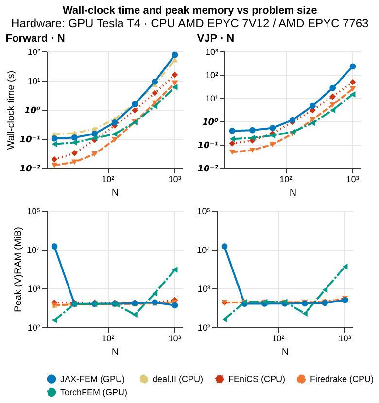
What does it cost? Wall-clock scaling of the forward and VJP passes with problem size \(N\) and the number of integration steps. Timings come from dedicated runners with no concurrent workloads; see the reliability note at the top of the page before reading absolute numbers.

Settings

Spatial Cost

Sweeps nx ∈ {16, 32, 64, 128, 256, 512, 1024}

{
  "physics": {
    "Lx": 2.0,
    "Ly": 1.0,
    "Q_total": 1.0,
    "rho_0": 0.5,
    "steps": 1,
    "nx": 16
  },
  "cost": {
    "n_trials": 3
  },
  "sweep": {
    "key": "nx",
    "values": [
      16,
      32,
      64,
      128,
      256,
      512,
      1024
    ]
  }
}

Temporal Cost

Sweeps steps ∈ {1}

{
  "physics": {
    "Lx": 2.0,
    "Ly": 1.0,
    "Q_total": 1.0,
    "rho_0": 0.5,
    "nx": 64,
    "steps": 1
  },
  "cost": {
    "n_trials": 3
  },
  "sweep": {
    "key": "steps",
    "values": [
      1
    ]
  }
}

Solver ranking

Solver	Forward time	VJP time
torch-fem	5.97 s @ N=1024	14.4 s @ N=1024
Firedrake	8.24 s @ N=1024	24.9 s @ N=1024
FEniCS	15.7 s @ N=1024	48.3 s @ N=1024
deal.II	52.2 s @ N=1024	—
JAX-FEM	76.2 s @ N=1024	227 s @ N=1024

Forward and VJP wall-clock time, each shown at the largest problem size N the solver completed for that pass; ranked by forward time (faster is better). The VJP time is one gradient from scratch, a forward plus an adjoint pass. Forward-only solvers have no VJP entry. See the reliability note above before comparing across devices.

Gradient

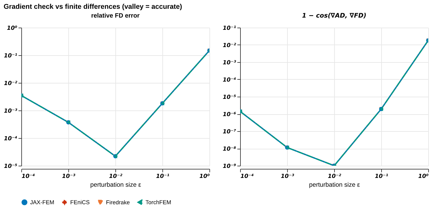
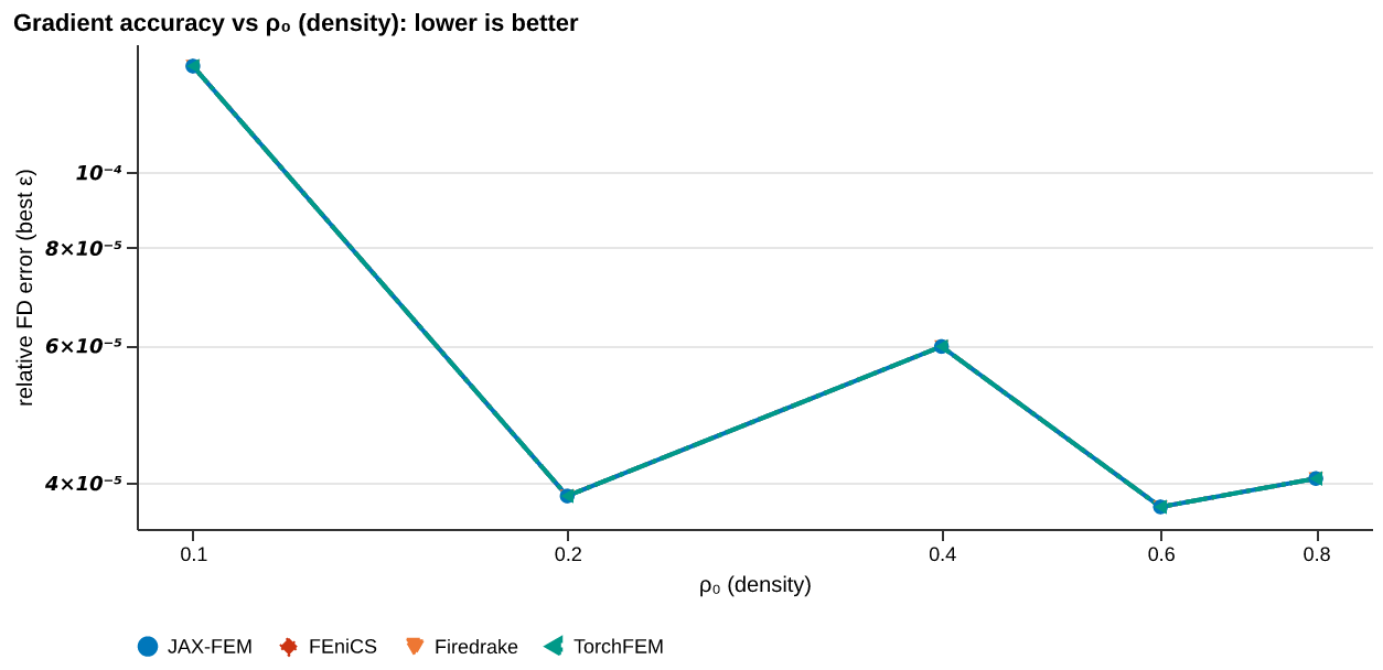
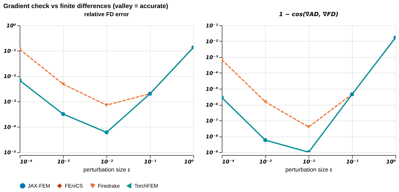
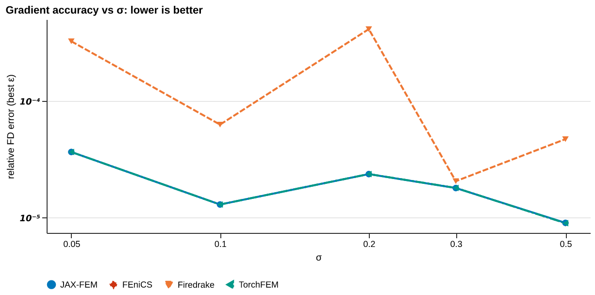
Is the gradient right? Gradient benchmarks compare each solver’s AD/adjoint gradient against a finite-difference ground truth. We report magnitude error (relative \(L^2\)) and direction agreement (cosine similarity) across parameter, resolution, and horizon sweeps. The horizon sweep in particular exposes how gradients degrade as the rollout lengthens.

Finite-Difference Check

FD gradient error vs step size \(\varepsilon\) (U-curves), AD/FD direction cosine, and gradient magnitude field panels.

Settings

{
  "ic": {
    "name": "random",
    "seed": 0
  },
  "physics": {
    "nx": 8,
    "ny": 4,
    "nz": 1,
    "Lx": 2.0,
    "Ly": 1.0,
    "Q_total": 1.0
  },
  "fd": {
    "eps_values": [
      1.0,
      0.1,
      0.01,
      0.001,
      0.0001
    ],
    "n_dirs": 6
  }
}

Parameter Sweep

Gradient norm, best-\(\varepsilon\) FD error, AD/FD direction cosine, and U-curves vs element density \(\rho_0\).

Settings

Sweeps rho_0 ∈ {0.1, 0.2, 0.4, 0.6, 0.8}

{
  "ic": {
    "name": "uniform",
    "seed": 0
  },
  "physics": {
    "nx": 8,
    "ny": 4,
    "nz": 1,
    "Lx": 2.0,
    "Ly": 1.0,
    "Q_total": 1.0,
    "rho_0": 0.1
  },
  "fd": {
    "eps_values": [
      1.0,
      0.1,
      0.01,
      0.001,
      0.0001
    ],
    "n_dirs": 6
  },
  "sweep": {
    "key": "rho_0",
    "values": [
      0.1,
      0.2,
      0.4,
      0.6,
      0.8
    ]
  }
}

Source Fd Check

FD gradient error vs \(\varepsilon\), AD/FD direction cosine, and gradient field panels for d(identification_error)/d(source).

Settings

{
  "ic": {
    "name": "gaussian_source"
  },
  "ic_key": "source",
  "output_key": "identification_error",
  "physics": {
    "nx": 8,
    "ny": 4,
    "nz": 1,
    "Lx": 2.0,
    "Ly": 1.0,
    "rho_0": 0.5,
    "target_from_two_gaussians": true,
    "ic_field": "source"
  },
  "fd": {
    "eps_values": [
      1.0,
      0.1,
      0.01,
      0.001,
      0.0001
    ],
    "n_dirs": 6
  }
}

Source Width Sweep

Gradient norm, best-\(\varepsilon\) FD error, AD/FD direction cosine, and U-curves vs source width \(\sigma\).

Settings

Sweeps sigma ∈ {0.05, 0.1, 0.2, 0.3, 0.5}

{
  "ic": {
    "name": "gaussian_source"
  },
  "ic_key": "source",
  "output_key": "identification_error",
  "physics": {
    "nx": 16,
    "ny": 8,
    "nz": 1,
    "rho_0": 0.5,
    "target_from_two_gaussians": true,
    "ic_field": "source"
  },
  "fd": {
    "eps_values": [
      0.1,
      0.01,
      0.001,
      0.0001
    ],
    "n_dirs": 4
  },
  "sweep": {
    "key": "sigma",
    "values": [
      0.05,
      0.1,
      0.2,
      0.3,
      0.5
    ],
    "ic_sweep": true
  }
}

Solver ranking

Solver	Best-ε FD error	1 − cosine
FEniCS	1.83e-05	2.21e-10
Firedrake	1.83e-05	2.21e-10
JAX-FEM	1.83e-05	2.21e-10
torch-fem	1.83e-05	2.21e-10

Ranked by the best-ε finite-difference error of the gradient (lower is more trustworthy); direction cosine near 1 confirms the gradient points the right way.

Optimization

Can you optimize through it? End-to-end optimization benchmarks run a gradient-based optimizer using each solver’s own gradients: recovery of initial conditions or physical parameters, topology optimization, and drag minimization. This is the ultimate test, since a gradient can pass the finite-difference check yet still fail to drive a full optimization loop.

Conductivity Recovery (L-BFGS)

Optimisation traces (loss vs iteration) and recovered conductivity fields vs the two-Gaussian ground truth, using L-BFGS.

Settings

{
  "ic": {
    "name": "uniform",
    "seed": 0
  },
  "physics": {
    "nx": 16,
    "ny": 8,
    "nz": 1,
    "Lx": 2.0,
    "Ly": 1.0,
    "rho_0": 0.5,
    "Q_total": 1.0,
    "compliance_key": "identification_error",
    "penalty_weight": 0.0,
    "x_min": 0.001,
    "snap_interval": 10,
    "target_rho_from_two_gaussians": true
  },
  "optim": {
    "max_iters": 1000
  },
  "optimizer": "bfgs"
}

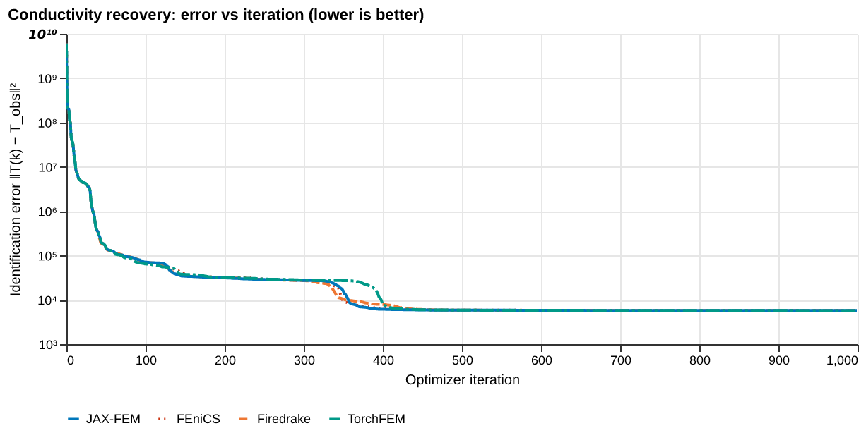
Solver ranking

Solver	Final error	Converged
torch-fem	5.69e+03	no
JAX-FEM	5.73e+03	no
FEniCS	5.73e+03	no
Firedrake	5.74e+03	no

Ranked by the final objective reached within the iteration budget (lower is better).